3  Results

3.1 Setup

This section loads the necessary tools and defines the visual style.

Code
knitr::opts_chunk$set(echo = TRUE, warning = FALSE, message = FALSE)

required_packages <- c(
  "tidyverse",
  "janitor",  
  "scales",      
  "ggrepel",     
  "ggalluvial",
  "RColorBrewer",
  "lubridate",
  "gridExtra",
  "tidyr"
)

install_and_load <- function(packages) {
  new_packages <- packages[!(packages %in% installed.packages()[, "Package"])]
  if (length(new_packages) > 0) {
    install.packages(new_packages)
  }
  invisible(lapply(packages, library, character.only = TRUE))
}

install_and_load(required_packages)

theme_swiss <- function() {
  theme_minimal(base_family = "Arial") +
    theme(
      plot.title = element_text(face = "bold", size = 16, color = "#2c3e50"),
      plot.subtitle = element_text(size = 12, color = "#7f8c8d"),
      axis.title = element_text(face = "bold", size = 10),
      legend.position = "bottom",
      panel.grid.minor = element_blank(),
      strip.text = element_text(face = "bold", hjust = 0)
    )
}
theme_set(theme_swiss())

3.2 Data Preparation

This section downloads the latest dataset from Swissvotes.

Code
DATA_DIR <- "data"
if (!dir.exists(DATA_DIR)) dir.create(DATA_DIR)

DATA_URL <- "https://swissvotes.ch/page/dataset/swissvotes_dataset.csv"
CODEBOOK_URL <- "https://swissvotes.ch/page/dataset/codebook-de.pdf"
REFS_URL <- "https://swissvotes.ch/page/dataset/kurzbeschreibung-de.pdf"

download_if_missing <- function(url, dest_path) {
  if (!file.exists(dest_path)) {
    download.file(url, dest_path, mode = "wb")
  }
}
download_if_missing(CODEBOOK_URL, file.path(DATA_DIR, "codebook.pdf"))
download_if_missing(REFS_URL, file.path(DATA_DIR, "references.pdf"))

file_pattern <- "DATASET.*\\.csv"
local_files <- list.files(DATA_DIR, pattern = file_pattern, full.names = TRUE)

if (length(local_files) > 0) {
  file_info <- file.info(local_files)
  target_file <- rownames(file_info)[which.max(file_info$mtime)]
  message(paste("Loading latest local file:", basename(target_file)))
} else {
  current_date_str <- format(Sys.Date(), "%d-%m-%Y") 
  new_filename <- paste0("DATASET CSV ", current_date_str, ".csv")
  target_file <- file.path(DATA_DIR, new_filename)
  
  message(paste("Downloading fresh dataset to:", new_filename))
  download.file(DATA_URL, target_file, mode = "wb")
}

votes <- read_delim(target_file, delim = ";", na = c(".", "", "9999"), show_col_types = FALSE) |>
  clean_names() |>
  mutate(
    date_vote = as.Date(datum, format = "%d.%m.%Y"),
    start_date = dmy(dat_start),
    submit_date = dmy(dat_submit),
    days_collected = as.numeric(difftime(submit_date, start_date, units = "days")),
    year = year(date_vote),
    across(where(is.character), ~ str_remove_all(., "'")),
    volkja_proz = as.numeric(volkja_proz),
    inserate_total = as.numeric(inserate_total),
    inserate_jaanteil = as.numeric(inserate_jaanteil),
    mediaton_tot = as.numeric(mediaton_tot),
    bet = as.numeric(bet),
    nrja = as.numeric(nrja),
    nrnein = as.numeric(nrnein),
    ktjaproz = as.numeric(ktjaproz),
    unter_quorum = as.numeric(unter_quorum), 
    unter_g = as.numeric(unter_g), 
    sammelfrist = as.numeric(sammelfrist)
  )

region_colors <- c(
  "German" = "#E74C3C",          
  "French" = "#3498DB", 
  "Italian" = "#27AE60",   
  "National" = "#95A5A6"        
)

outcome_colors <- c(
  "Accepted" = "#27AE60", 
  "Rejected" = "#E74C3C"
)

canton_meta <- tibble(
  canton_code = c("ZH", "BE", "LU", "UR", "SZ", "OW", "NW", "GL", "ZG", "FR", "SO", "BS", "BL", "SH", "AR", "AI", "SG", "GR", "AG", "TG", "TI", "VD", "VS", "NE", "GE", "JU"),
  region = c("German", "German", "German", "German", "German", "German", "German", "German", "German", "French", "German", "German", "German", "German", "German", "German", "German", "German", "German", "German", "Italian", "French", "French", "French", "French", "French")
)

3.3 Mobilization: Getting on the Ballot

Before a vote can take place, committees must succeed in a race against the clock. Whether launching an Optional Referendum to challenge a new parliamentary law or a Popular Initiative to propose a constitutional amendment, the requirements are demanding. Referendum committees face a 100-day sprint to gather 50,000 signatures, while Initiative committees must sustain an 18-month effort to validate 100,000 signatures.

This chart illustrates these mobilization dynamics by showing how close campaigns came to their respective legal deadlines.

Code
plot_data_all <- votes |>
  filter(year(date_vote) >= 2000) |>
  filter(rechtsform %in% c(2, 3), !is.na(start_date), !is.na(submit_date)) |>
  mutate(
    legal_deadline = ifelse(sammelfrist > 0 & !is.na(sammelfrist), 
                            sammelfrist, 
                            ifelse(rechtsform == 2, 100, 548)),
    
    days_relative = days_collected - legal_deadline, 
    
    theme = case_when(
      d1e1 == 1 ~ "State Order", d1e1 == 2 ~ "Foreign Policy", d1e1 == 3 ~ "Security",
      d1e1 == 4 ~ "Economy", d1e1 == 5 ~ "Agriculture", d1e1 == 6 ~ "Public Finance",
      d1e1 == 7 ~ "Energy", d1e1 == 8 ~ "Transport", d1e1 == 9 ~ "Environment",
      d1e1 == 10 ~ "Social Policy", d1e1 == 11 ~ "Education", d1e1 == 12 ~ "Culture",
      TRUE ~ "Other"
    ),
    
    type_label = ifelse(rechtsform == 2, 
                        "Optional Referendum\n(Deadline: ~100 Days)", 
                        "Popular Initiative\n(Deadline: ~18 Months)")
  ) |>
  filter(days_collected >= 0)

summary_all <- plot_data_all |>
  group_by(theme, type_label) |>
  summarise(
    avg_diff = mean(days_relative),
    min_diff = min(days_relative),
    max_diff = max(days_relative),
    count = n(),
    .groups = "drop"
  ) |>
  filter(count >= 2)

overtime_data <- summary_all |>
  filter(max_diff > 0)

limit_range <- tibble(
  type_label = rep(c("Optional Referendum\n(Deadline: ~100 Days)", 
                     "Popular Initiative\n(Deadline: ~18 Months)"), each = 2),
  x_limit = c(-25, 85, -450, 100) 
)

ggplot(summary_all, aes(y = reorder(theme, avg_diff))) +
  
  geom_blank(data = limit_range, aes(x = x_limit, y = NULL)) +

  geom_linerange(aes(xmin = min_diff, xmax = max_diff), color = "grey70", size = 1) +
  
  geom_segment(
    data = overtime_data,
    aes(x = 0, xend = max_diff, y = theme, yend = theme), 
    color = "#E74C3C", size = 1.2
  ) +
  
  geom_point(aes(x = avg_diff, color = type_label), size = 4) +
  
  geom_vline(xintercept = 0, linetype = "dashed", color = "black") +
  
  facet_wrap(~type_label, scales = "free_x") +
  
  scale_x_continuous(
    breaks = scales::pretty_breaks(n = 6)
  ) +

  scale_color_manual(values = c("#E74C3C", "#2C3E50")) +
  
  labs(
    title = "Mobilization Variance by Policy Area (2000-Present)",
    subtitle = "Points represent the average collection time. Bars show the range (fastest to slowest).\nDashed lines indicate the legal deadline.\nRed segments indicate overtime beyond the standard deadline\n(primarily due to COVID-19 extensions).",
    x = "Days Relative to Deadline (Negative = Early, Positive = Overtime)",
    y = NULL
  ) +
  
  theme(
    strip.text = element_text(face = "bold", size = 11, margin = margin(b = 15)),
    legend.position = "none",
    panel.grid.major.y = element_line(linetype = "dotted"),
    plot.margin = margin(t = 20, r = 10, b = 10, l = 10) 
  ) +
  
  coord_cartesian(clip = "off") +
  
  annotate("text", x = 0, y = 13.2, label = "Deadline", 
           vjust = 0, size = 3.5, fontface = "italic", color = "black")

The ‘Pressure’ of Democracy: Signature Collection Speed relative to Deadline

It reveals two distinct speeds of political action. On the left, Optional Referendums operate under extreme time constraints. The tight clustering near the zero-line confirms that challenging a law is a high-pressure sprint where committees need almost every available day of the 100-day limit. The significant red outliers in Foreign Policy and Security underscore this fragility: they represent the campaigns against the Indonesia Trade Agreement and new Fighter Jets, where the government had to officially pause the legal countdown during the COVID-19 lockdown. Because street collection is so vital to Swiss democracy, the system effectively halted without it.

On the right, Popular Initiatives reveal which topics resonate most with the public. The long grey lines stretching to the left for Social Policy and Foreign Policy indicate that these campaigns often finish months ahead of schedule. These issues tend to be highly emotional and tangible (e.g., pensions, national identity), allowing organizers to mobilize voters quickly. In contrast, initiatives regarding Public Finance or Energy consistently press right up against the deadline, utilizing the full 18-month period. These topics are often more technical or abstract, making them harder to “sell” to passersby. Consequently, committees in these areas must work harder and longer to convince citizens that the issue is urgent enough to warrant a signature.

3.4 The Campaign: Money & Media

Once a proposal qualifies for the ballot, the signature lists are filed away and the battle for public opinion begins. This phase is defined by two powerful external forces: Financial Resources (Advertising) and Information Flow (Media Coverage).

Does Switzerland have a “pay-to-play” democracy where the richest campaign always wins? Or does the “Fourth Estate” (the media) hold the real power to sway voters? The following visualizations test these assumptions by mapping advertising dominance and media sentiment against the actual decisions made at the ballot box.

3.4.1 Can Money Buy Votes?

This scatter plot investigates the correlation between Advertising Dominance (share of total print ads) and Electoral Success. By highlighting extreme campaigns that spent heavily but lost (“Money Pits”) versus those that spent little but won (“Underdogs”), we test the limits of financial influence.

Code
scatter_data <- votes |>
  filter(year(date_vote) >= 2000) |>
  select(
    title = titel_kurz_e,
    volkja_proz,          
    annahme,              
    inserate_total,       
    inserate_jaanteil     
  ) |>
  filter(!is.na(inserate_jaanteil), !is.na(volkja_proz)) |>
  mutate(
    outcome_label = ifelse(annahme == 1, "Accepted", "Rejected"),
  )

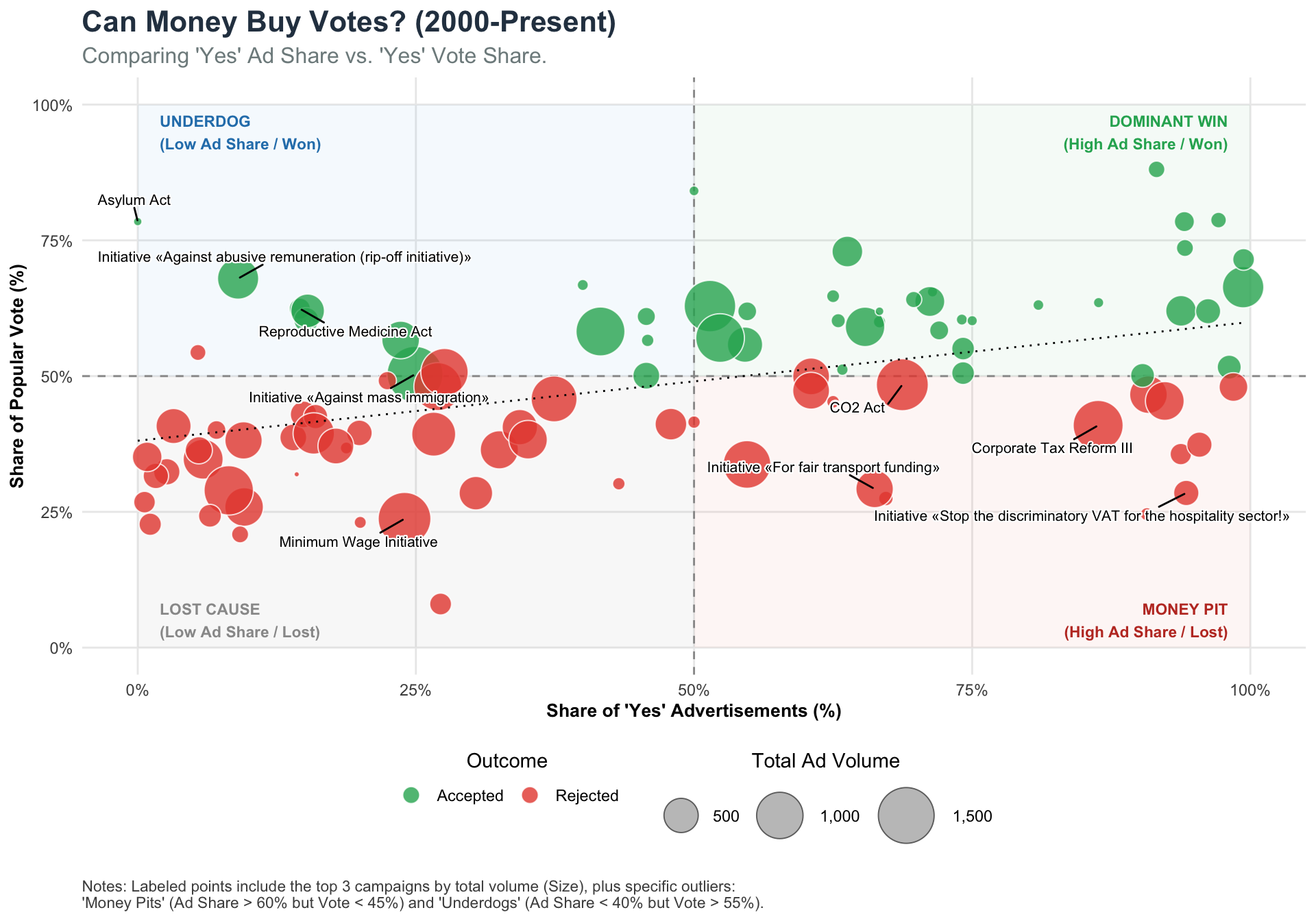
money_pits <- scatter_data |>
  filter(inserate_jaanteil > 60 & volkja_proz < 45) |>
  slice_max(order_by = inserate_total, n = 3)

underdogs <- scatter_data |>
  filter(inserate_jaanteil < 40 & volkja_proz > 55) |>
  slice_max(order_by = volkja_proz, n = 3)

behemoths <- scatter_data |>
  slice_max(order_by = inserate_total, n = 3)

labels_final <- bind_rows(money_pits, underdogs, behemoths) |> distinct(title, .keep_all = TRUE)

ggplot(scatter_data, aes(x = inserate_jaanteil, y = volkja_proz)) +
  
  annotate("rect", xmin = 50, xmax = 100, ymin = 50, ymax = 100, fill = "#27AE60", alpha = 0.05) +
  annotate("rect", xmin = 50, xmax = 100, ymin = 0, ymax = 50, fill = "#E74C3C", alpha = 0.05) +
  annotate("rect", xmin = 0, xmax = 50, ymin = 50, ymax = 100, fill = "#3498DB", alpha = 0.05) +
  annotate("rect", xmin = 0, xmax = 50, ymin = 0, ymax = 50, fill = "grey50", alpha = 0.05) +

  geom_hline(yintercept = 50, linetype = "dashed", color = "grey60") +
  geom_vline(xintercept = 50, linetype = "dashed", color = "grey60") +
  
  annotate("text", x = 98, y = 98, label = "DOMINANT WIN\n(High Ad Share / Won)", hjust = 1, vjust = 1, fontface = "bold", size = 3, color = "#27AE60") +
  annotate("text", x = 98, y = 2, label = "MONEY PIT\n(High Ad Share / Lost)", hjust = 1, vjust = 0, fontface = "bold", size = 3, color = "#C0392B") +
  annotate("text", x = 2, y = 98, label = "UNDERDOG\n(Low Ad Share / Won)", hjust = 0, vjust = 1, fontface = "bold", size = 3, color = "#2980B9") +
  annotate("text", x = 2, y = 2, label = "LOST CAUSE\n(Low Ad Share / Lost)", hjust = 0, vjust = 0, fontface = "bold", size = 3, color = "grey60") +

  geom_point(aes(size = inserate_total, fill = outcome_label), shape = 21, color = "white", stroke = 0.5, alpha = 0.8) +
  
  geom_text_repel(
    data = labels_final,
    aes(label = title),
    size = 2.8,
    min.segment.length = 0,
    box.padding = 0.6,
    max.overlaps = Inf,
    bg.color = "white", 
    bg.r = 0.15
  ) +

  geom_smooth(method = "lm", color = "black", se = FALSE, linetype = "dotted", size = 0.5) +
  
  scale_x_continuous(labels = percent_format(scale = 1), limits = c(0, 100)) +
  scale_y_continuous(labels = percent_format(scale = 1), limits = c(0, 100)) +
  scale_size_continuous(range = c(1, 14), labels = label_comma(), name = "Total Ad Volume") +
  scale_fill_manual(values = outcome_colors, name = "Outcome") +
  
  labs(
    title = "Can Money Buy Votes? (2000-Present)",
    subtitle = "Comparing 'Yes' Ad Share vs. 'Yes' Vote Share.",
    caption = "Notes: Labeled points include the top 3 campaigns by total volume (Size), plus specific outliers:\n'Money Pits' (Ad Share > 60% but Vote < 45%) and 'Underdogs' (Ad Share < 40% but Vote > 55%).",
    x = "Share of 'Yes' Advertisements (%)",
    y = "Share of Popular Vote (%)"
  ) +
  theme(
    plot.caption = element_text(hjust = 0, size = 8.5, color = "grey30", margin = margin(t = 10)),
    legend.box = "horizontal",
  ) +
  
  guides(
    size = guide_legend(
      title.position = "top", 
      title.hjust = 0.5,
      override.aes = list(fill = "grey70", color = "grey30")
    ),
    fill = guide_legend(
      title.position = "top", 
      title.hjust = 0.5,
      override.aes = list(size = 4) 
    )
  )

Impact of Ad Spending on Vote Outcome

The visualization challenges the cynical view that Swiss democracy is simply “for sale.” While the trend line shows a slight positive correlation, implying that visibility certainly helps, the relationship is far from decisive. The existence of massive “Money Pits” (bottom-right) demonstrates the limits of financial power. Campaigns like the Corporate Tax Reform III or the CO2 Act dominated the advertising landscape with massive budgets yet still faced rejection by voters. Conversely, the “Underdog” quadrant (top-left) proves that high-resonance topics, such as the initiative for the Reproductive Medicine Act and the Asylum Act can secure landslide victories purely on the strength of public sentiment, with almost no advertising budget at all. Ultimately, money appears to amplify a message, but it cannot manufacture consent for a policy the public fundamentally dislikes. Furthermore, the large size of the bubbles in the “Rejected” zones suggests a pattern of defensive spending. Massive advertisement is often deployed as a last-ditch effort to save sinking campaigns, rather than a proactive display of strength.

3.4.2 The “Fourth Estate” Disconnect

In a direct democracy, the media acts as a critical bridge between policy and the public, yet this relationship is not always aligned. This chart quantifies the “Gap Score” by comparing the tone of media coverage against the final popular vote, revealing whether the press reflects or contradicts the public will. The visualization ranks the most significant divergences since 2000, highlighting moments where the public embraced proposals despite negative coverage or rejected government projects that the media had strongly endorsed.

Code
gap_data <- votes |>
  filter(year(date_vote) >= 2000) |>
  select(title = titel_kurz_e, volkja_proz, annahme, mediaton_tot) |>
  filter(!is.na(mediaton_tot), !is.na(volkja_proz)) |>
  mutate(
    outcome_label = ifelse(annahme == 1, "Accepted", "Rejected"),
    media_normalized = (mediaton_tot + 100) / 2,
    gap = volkja_proz - media_normalized,
    title_short = str_wrap(title, width = 35) 
  )

plot_data <- gap_data |>
  mutate(
    category_raw = case_when(
      gap > 0 ~ "POPULIST SENTIMENT\n(People more Positive than Media)",
      gap < 0 ~ "ESTABLISHMENT FAILURE\n(Media more Positive than People)"
    )
  ) |>
  mutate(category = fct_reorder(category_raw, gap, .desc = TRUE)) |>
  group_by(category) |>
  slice_max(abs(gap), n = 10) |>
  ungroup()

ggplot(plot_data, aes(x = gap, y = reorder(title_short, gap))) +
  
  geom_segment(aes(x = 0, xend = gap, y = title_short, yend = title_short), 
               color = "grey70", size = 0.8) +
  
  geom_point(aes(color = outcome_label), size = 4) +
  
  geom_vline(xintercept = 0, linetype = "solid", color = "black") +
  
  facet_wrap(~category, ncol = 1, scales = "free_y") +
  
  scale_x_continuous(limits = c(-50, 50), breaks = c(-40, -20, 0, 20, 40)) +
  scale_color_manual(values = outcome_colors, 
                     name = "Actual Outcome") +
  
  labs(
    title = "The Media-Public Disconnect (2000-Present)",
    subtitle = "Gap = Popular Vote % minus Normalized Media Tone.\nShowing the 10 most extreme divergences where media and public opinion clashed.",
    x = "← Media was more Positive           Gap Score           People were more Positive →",
    y = NULL,
  ) +
  
  theme(
    strip.text = element_text(face = "bold", size = 10, color = "black"),
    strip.background = element_rect(fill = "grey95", color = NA),
    panel.grid.major.y = element_blank(),
    plot.margin = margin(t = 20, r = 10, b = 10, l = 10),
    axis.text.y = element_text(size = 9, lineheight = 0.8),
    axis.title.x = element_text(face = "bold", size = 10, margin = margin(t = 10))
  )

The Media-Public Gap

The top section, “Populist Sentiment,” reveals that voters frequently disregard media skepticism on issues regarding law and order or social morality. The most extreme example, the Initiative against Pedophiles, illustrates this divergence. While media coverage was largely negative, likely focusing on legal conflicts and proportionality, the public voted overwhelmingly in favor. A similar pattern appears in votes regarding Police Measures and Border Control, where the electorate consistently prioritizes stricter security measures even when the media views them with caution.

The bottom section, “Establishment Failure,” highlights the opposite dynamic. Here, the media tends to align with government experts and institutions on complex, structural reforms, such as the CO2 Act or Pension Reform. While the press coverage largely reflected a consensus on the long-term necessity of these measures, voters rejected them. This suggests a disconnect between the media’s focus on expert-driven policy solutions and the citizens’ hesitation to accept the immediate financial burdens or lifestyle changes those solutions require.

3.5 Participation: The Voice of the People

Voting in Switzerland is frequent (typically four Sundays per year) but not mandatory, with one notable cantonal exception*. This structure creates unique participation patterns compared to other democracies where elections are rare but high-stakes events.

*We will get to that soon.

3.5.1 The Evolution of Engagement

The following chart explores the historical evolution of voter engagement, tracing the fluctuations in turnout through the key defining moments of Switzerland’s democratic history.

Code
annual_turnout <- votes |>
  select(anr, datum, year, turnout = bet) |>
  filter(!is.na(turnout), !is.na(year)) |>
  group_by(year) |>
  summarize(
    avg_turnout = mean(turnout, na.rm = TRUE),
    min_turnout = min(turnout, na.rm = TRUE),
    max_turnout = max(turnout, na.rm = TRUE),
    n_votes = n()
  )

highlight_meta <- tibble(
  year = c(1933, 1959, 1971, 1992),
  label = c("1930s: Defense of Democracy\n(Turnout Peak)", 
            "1959: Magic Formula\n(Consensus Begins)", 
            "1971: Electorate Expansion\n(Women's Suffrage)", 
            "1992: EEA Vote\n(The 'Wake Up' Spike)")
)

highlights <- annual_turnout |>
  inner_join(highlight_meta, by = "year")

ggplot(annual_turnout, aes(x = year, y = avg_turnout)) +
  
  geom_linerange(aes(ymin = min_turnout, ymax = max_turnout), 
                 color = "#2c3e50", alpha = 0.3, size = 0.5) +
  
  geom_smooth(color = "#5D6D7E", fill = "#5D6D7E", alpha = 0.15, size = 1, span = 0.4) +
  
  geom_point(color = "#2c3e50", size = 1.5, alpha = 0.6) +
  
  geom_point(data = highlights, color = "#E74C3C", size = 4, shape = 1) +
  
  geom_label_repel(
    data = highlights,
    aes(label = label),
    
    segment.color = NA,      
    
    nudge_y = c(13, -23, -23, 40), 
    nudge_x = c(0, -5, 0, 0),
    
    color = "#E74C3C",
    fontface = "bold",
    size = 3.5,
    box.padding = 0.5
  ) +

  scale_y_continuous(labels = percent_format(scale = 1), limits = c(0, 100)) +
  scale_x_continuous(breaks = seq(1850, 2025, by = 25)) + 
  
  labs(
    title = "Historical Turnout Ranges (1848-2025)",
    subtitle = "Vertical bars show the annual range (lowest to highest). The grey curve represents the smoothed long-term trend.",
    x = "Year",
    y = "Voter Turnout (%)"
  )

Annual Voter Turnout Ranges (1879-2025)

The historical trajectory of Swiss voter turnout tells a story of changing civic identity. The peak in the 1930s reflects the era of “Spiritual National Defense,” where high participation was viewed as a patriotic duty to differentiate Swiss democracy from the rising tide of fascism in neighboring Germany and Italy.

Post-WWII, a long decline began. This paradoxically stems from political stability. The introduction of the “Magic Formula” in 1959 (a permanent coalition government sharing power between the four major parties) replaced political conflict with consensus. With the outcome of elections becoming less volatile, the urgency to vote decreased. The visual dip in 1971 marks a statistical adjustment rather than a sudden loss of interest. The introduction of women’s suffrage doubled the electorate overnight and it took time for the new participation rates to stabilize.

The modern era is defined by the 1992 European Economic Area (EEA) vote. This massive spike, reaching nearly 80%, signaled a shift to “selective participation.” Today, the average hovers around 45-50%, but this figure is misleading if compared to nations with infrequent elections. Since Swiss citizens are called to the polls up to four times a year, maintaining high turnout for every single ballot is difficult. Consequently, the electorate is highly fluid. Citizens pick and choose when to participate based on the specific issues at stake. While the turnout for any single Sunday may be low, the percentage of Swiss who vote at least once a year is significantly higher. Moreover, as the wide vertical ranges in the chart demonstrate, modern turnout is highly volatile. Participation spikes for high-stakes, emotional issues (like COVID laws) but drops significantly for technical administrative votes.

3.5.2 The “Röstigraben” of Participation

While national trends fluctuate, regional habits remain surprisingly sticky. Swiss politics is often defined by the Röstigraben (literally “Hash Brown Ditch”). Much has been said about this cultural border separating the German-speaking majority from the French- and Italian-speaking minorities.

The following boxplot reveals that this divide extends beyond policy preferences to civic duty itself, showing a persistent difference in voter engagement between the linguistic communities.

Code
canton_turnout <- votes |>
  select(anr, ends_with("_bet")) |>
  pivot_longer(
    cols = ends_with("_bet"),
    names_to = "canton_code_raw",
    values_to = "turnout"
  ) |>
  mutate(
    turnout = as.numeric(turnout),
    canton_code = str_to_upper(str_remove(canton_code_raw, "_bet"))
  ) |>
  filter(!is.na(turnout)) |>
  left_join(canton_meta, by = "canton_code")

national_turnout <- votes |>
  select(anr, turnout = bet) |>
  mutate(
    turnout = as.numeric(turnout),
    canton_code = "CH",
    region = "National"
  ) |>
  filter(!is.na(turnout))

plot_data <- bind_rows(canton_turnout, national_turnout)

canton_order <- plot_data |>
  group_by(canton_code) |>
  summarize(median_turnout = median(turnout, na.rm = TRUE)) |>
  arrange(median_turnout) |>
  pull(canton_code)

axis_face <- ifelse(canton_order == "CH", "bold", "plain")

plot_data |>
  mutate(canton_code = factor(canton_code, levels = canton_order)) |>
  ggplot(aes(x = turnout, y = canton_code, fill = region)) +
  
  geom_boxplot(outlier.shape = NA, alpha = 0.8, color = "#2c3e50", size = 0.3) +
  
  scale_fill_manual(values = region_colors) +
  scale_x_continuous(labels = percent_format(scale = 1), limits = c(0, 100)) +
  
  labs(
    title = "Turnout by Canton and Language Region",
    subtitle = "Ordered by median turnout. 'CH' represents the national average.",
    x = "Voter Turnout (%)",
    y = "Canton",
    fill = "Region"
  ) +
  theme(
    legend.position = "top",
    axis.text.y = element_text(size = 9, face = axis_face),
    panel.grid.major.y = element_blank()
  )

Median Voter Turnout by Canton (1848-2025) split by Language Region

The chart confirms that the Röstigraben is not just a metaphor for policy disagreement, but a structural reality of civic life. The visualization reveals a striking stratification: German-speaking cantons (red) exclusively occupy the top of the chart, while French (blue) and Italian (green) cantons cluster at the bottom.

Two key insights stand out. First, Schaffhausen (SH) sits alone at the very top as an institutional outlier. Its high turnout is not due to superior enthusiasm, but to the fact that it is the only canton that still enforces compulsory voting, levying a small fine on citizens who fail to cast a ballot. Second, the broader split reflects a deep sociological difference. In the German-speaking tradition, voting is culturally ingrained as a civic duty (or Pflicht). It is viewed as a mandatory contribution to the collective, much like paying taxes. In contrast, “Latin Switzerland” tends to view voting as a political right, a privilege to be exercised when one is inspired, but optional when one is not. This persistent gap exacerbates the political dominance of the German majority, as the linguistic minorities are not only outnumbered by population but also by engagement.

3.6 Vote Theme: The Shifting Agenda

What issues drive the Swiss to the ballot box? Over the last 177 years, the focus of direct democracy has evolved from foundational questions of statehood to a diverse array of modern challenges.

This chart maps the history of federal votes by policy domain, visualizing the changing thematic landscape of Swiss politics.

Code
policy_labels <- c(
  `1` = "1: State Order",
  `2` = "2: Foreign Policy",
  `3` = "3: Security Policy",
  `4` = "4: Economy",
  `5` = "5: Agriculture",
  `6` = "6: Public Finances",
  `7` = "7: Energy",
  `8` = "8: Transport",
  `9` = "9: Environment",
  `10` = "10: Social Policy",
  `11` = "11: Education/Research",
  `12` = "12: Culture/Religion/Media"
)

pal_set1 <- brewer.pal(9, "Set1")
pal_dark2 <- brewer.pal(8, "Dark2")
pal_set1[6] <- "#66A61E"

strong_domain_colors <- c(pal_set1[1:9], pal_dark2[1:3])
names(strong_domain_colors) <- unname(policy_labels)

all_colors <- c(
  strong_domain_colors,
  "Other" = "grey95",
  "NA_vote" = "transparent"
)

vote_data <- votes |>
  filter(!is.na(date_vote)) |>
  mutate(
    month = as.numeric(format(date_vote, "%m"))
  ) |>
  mutate(
    vote_quarter = factor(case_when(
      month %in% c(2, 3)    ~ "Q1 (Feb/Mar)",
      month %in% c(5, 6)    ~ "Q2 (May/Jun)",
      month %in% c(9, 10)   ~ "Q3 (Sep/Oct)",
      month %in% c(11, 12)  ~ "Q4 (Nov/Dec)",
      TRUE                  ~ "Other"
    ), levels = c("Q1 (Feb/Mar)", "Q2 (May/Jun)", "Q3 (Sep/Oct)", "Q4 (Nov/Dec)", "Other"))
  ) |>
  mutate(
    policy_domain = factor(d1e1,
                           levels = names(policy_labels),
                           labels = unname(policy_labels))
  ) |>
  filter(vote_quarter != "Other") |>
  group_by(year, vote_quarter) |>
  mutate(vote_index = row_number()) |>
  ungroup()

max_votes <- max(vote_data$vote_index, na.rm = TRUE)
min_year <- min(vote_data$year)
max_year <- max(vote_data$year)
all_quarters <- levels(vote_data$vote_quarter)
all_quarters <- all_quarters[all_quarters != "Other"]

complete_grid <- expand_grid(
  year = min_year:max_year,
  vote_quarter = all_quarters
)

plot_data_complete <- complete_grid |>
  left_join(vote_data, by = c("year", "vote_quarter")) |>
  arrange(year, vote_quarter) |>
  mutate(x_label = fct_inorder(paste(year, vote_quarter)))

facet_levels <- levels(vote_data$policy_domain)

plot_data_faceted <- crossing(
    plot_data_complete,
    facet_domain = facet_levels
  ) |>
  mutate(
    highlight_color = case_when(
      is.na(policy_domain) ~ "NA_vote",
      as.character(policy_domain) == facet_domain ~ as.character(policy_domain),
      TRUE ~ "Other"
    )
  ) |>
  mutate(
    is_highlight = (highlight_color != "Other" & highlight_color != "NA_vote")
  ) |>
  group_by(x_label, facet_domain) |>
  arrange(desc(is_highlight), vote_index) |>
  mutate(
    y_stack = if_else(is.na(vote_index), NA_real_, as.numeric(row_number()))
  ) |>
  ungroup()

year_breaks_df <- plot_data_complete |>
  filter(vote_quarter == "Q1 (Feb/Mar)" & year %% 10 == 0) |>
  select(x_label, year) |>
  distinct()

ggplot(
    plot_data_faceted, 
    aes(x = x_label, y = y_stack, fill = highlight_color)
  ) +
    geom_tile(color = "white", linewidth = 0.05, height = 1) +
    
    facet_wrap(~ factor(facet_domain, levels = facet_levels), ncol = 1) + 
    
    scale_fill_manual(values = all_colors, guide = "none", na.value = "transparent") +
    
    scale_x_discrete(
      breaks = year_breaks_df$x_label,
      labels = year_breaks_df$year,
      drop = FALSE
    ) +
    
    scale_y_continuous(breaks = c(1, 3, 5, 7, 9)) +
    
    labs(
      title = "Federal Votes Over Time by Policy Domain",
      subtitle = "Each panel highlights one policy domain in color against the backdrop of all other votes (grey).",
      x = "Year",
      y = "Votes per Session"
    ) +
    
    theme(
      axis.text.x = element_text(angle = 45, vjust = 0.5, size = 8),
      panel.grid = element_blank(),
      strip.background = element_rect(fill = "grey90", color = NA),
      strip.text = element_text(face = "bold", size = 9, hjust = 0.5),
      panel.spacing = unit(0.5, "lines")
    )

Thematic Composition of Federal Votes (1848-2025)

This chart visualizes the growing demands placed on the Swiss electorate. Thematically, the agenda has shifted from narrow constitutional questions to a broad spectrum of issues regulating the daily existence and well-being of the population. In the 19th century (far left), the focus was singular and dominated almost exclusively by State Order (Panel 1) and the Economy (Panel 4), as the young federation established its foundations. As we move right, this focus splinters into a diverse array of modern challenges. Social Policy (Panel 10) has exploded to become the dominant battleground of the 21st century. Simultaneously, diverse topics, such as Environment, Education and Culture, have emerged from obscurity to become part of the national debate, proving that direct democracy has evolved to cover nearly every aspect of daily life.

The most striking trend, however, is the sheer volume of decision-making required. The visual density on the right reveals an acceleration of democracy. Voting is no longer a sporadic occurrence but a constant feature of civic life. The height of the stacks indicates a densification of the ballot, where voters frequently face “Super Sundays” containing four or five distinct proposals. This trend mirrors the growth of the modern administrative state, where the mechanisms of direct democracy have scaled to match the increasing frequency and complexity of legislation, demanding significantly higher engagement from every citizen.

3.7 The “Elite-People Gap”

Before every federal vote, Swiss mailboxes receive the official “Voting Pamphlet” (Bundesbüchlein), a direct line of communication from the government to the citizen. In this booklet, the Federal Council and Parliament (“National Council”) present their arguments and issue a formal voting recommendation, either a Yes or a No.

But does the electorate listen? Does a unanimous Parliament guarantee a “Yes” from the people or is there a disconnect between the political elite in Bern and the voters? The following chart visualizes this relationship by comparing the consensus level in the National Council against the final popular verdict.

Code
gap_data <- votes |>
  mutate(
    people_yes = volkja_proz,
    
    nc_total = nrja + nrnein,
    parl_consensus = (nrja / nc_total) * 100,
    
    Outcome = factor(
      ifelse(annahme == 0, "Rejected", "Accepted"),
      levels = c("Accepted", "Rejected")
    )
  ) |>
  filter(
    !is.na(parl_consensus), 
    !is.na(people_yes),
    !is.na(Outcome),
    nc_total > 0
  )

ggplot(gap_data, aes(x = parl_consensus, y = people_yes)) +
  
  geom_abline(intercept = 0, slope = 1, color = "grey80", linetype = "solid", size = 0.5) +
  geom_hline(yintercept = 50, linetype = "dashed", color = "grey60") +
  
  annotate("text", x = 95, y = 5, label = "The 'Elite Disconnect'\n(Parliament Yes, People No)", 
           color = "#E74C3C", size = 3.5, fontface = "italic", hjust = 1) +
  annotate("text", x = 10, y = 95, label = "Populist Surprise\n(Parliament No, People Yes)", 
           color = "#3498DB", size = 3.5, fontface = "italic", hjust = 0) +
  
  geom_point(
    aes(color = Outcome),
    size = 2.5,
    alpha = 0.5
  ) +
  
  geom_smooth(method = "lm", color = "black", size = 0.5, se = FALSE, linetype = "dotdash") +
  
  scale_x_continuous(labels = percent_format(scale = 1), limits = c(0, 100)) +
  scale_y_continuous(labels = percent_format(scale = 1), limits = c(0, 100)) +
  scale_color_manual(values = outcome_colors) +
  
  labs(
    title = "Does Parliament Represent the People?",
    subtitle = "Comparison of 'Yes' vote share in the National Council vs. the Popular Vote.",
    x = "Parliamentary Consensus (% Yes in National Council)",
    y = "Popular Vote (% Yes from Citizens)",
    color = "Outcome",
    caption = "Note: Red points above the 50% line indicate votes that won the Popular Majority\nbut failed to reach the required Cantonal Majority ('Ständemehr')."
  )

Parliamentary Consensus vs. Popular Vote (1848-2025)

This scatter plot reveals a fundamental asymmetry in Swiss democracy. The strong diagonal trend confirms that Parliament is generally a reliable barometer of the public mood. When the National Council agrees, citizens usually follow. However, the cluster of red points in the bottom-right demonstrates that a unified political establishment is not immune to a popular veto, as seen when voters rejected votes, like the CO2 Act or the e-ID Act, despite near-unanimous parliamentary support.

Conversely, the empty top-left corner proves that while the people possess a powerful “emergency brake” to stop the government, they rarely succeed in forcing new legislation through against the united advice of Parliament.

3.8 The Political Landscape: Results & Regions

We have analyzed the mobilization, the campaigns, and the participation. Now, we look at the results. How do these 650+ votes actually turn out and what do they reveal about the internal geography of Swiss politics?

3.8.1 The Legislative Funnel

In Swiss direct democracy, the origin of a proposal largely determines its fate. Not all votes are created equal. In fact, proposals crafted by the government face a very different path than those launched by citizens.

The Mandatory Referendum (constitutional changes proposed by Parliament) and the Optional Referendum (challenges to new laws) act as checks on the system. In contrast, the Popular Initiative allows citizens to step on the gas pedal and propose entirely new ideas. The following alluvial diagram tracks this “legislative funnel,” mapping the flow of votes from their legal instrument, through their policy domain, to their final verdict (Accepted or Rejected).

Code
alluvial_data <- votes |>
  filter(year >= 1990) |>
  mutate(
    legal_form = case_when(
      rechtsform == 1 ~ "Mandatory Ref.",
      rechtsform == 2 ~ "Optional Ref.",
      rechtsform == 3 ~ "Popular Initiative",
      TRUE ~ "Other"
    ),
    policy_area = case_when(
      d1e1 %in% c(1, 2, 3, 11) ~ "State & Security",
      d1e1 %in% c(4, 5, 6) ~ "Economy & Infra",
      d1e1 %in% c(8, 9, 10) ~ "Social & Culture",
      d1e1 == 7 ~ "Environment",
      TRUE ~ "Other"
    ),
    outcome_label = ifelse(annahme == 1, "Accepted", "Rejected")
  ) |>
  filter(legal_form != "Other") |>
  mutate(
    legal_form = fct_infreq(legal_form),
    policy_area = fct_infreq(policy_area),
    outcome_label = fct_infreq(outcome_label)
  ) |>
  group_by(legal_form, policy_area, outcome_label) |>
  summarise(freq = n(), .groups = "drop")

ggplot(alluvial_data, aes(y = freq, axis1 = legal_form, axis2 = policy_area, axis3 = outcome_label)) +
  
  geom_alluvium(aes(fill = legal_form), width = 1/12, alpha = 0.7, color = "white") +
  
  geom_stratum(width = 1/12, fill = "grey90", color = "grey20") +
  
  geom_text(stat = "stratum", aes(label = after_stat(stratum)), size = 3, family = "Arial") +
  
  scale_fill_brewer(palette = "Dark2", name = "Legal Instrument") +
  
  scale_x_discrete(limits = c("Instrument", "Topic", "Outcome"), expand = c(.05, .05)) +
  
  labs(
    title = "The Fate of Legislation (1990-2024)",
    subtitle = "Ordered by Frequency (Most Frequent at the Top)",
    y = "Number of Votes"
  ) +

  theme(
    axis.text.y = element_blank(),
    axis.ticks = element_blank(),
    panel.grid = element_blank(),
  )

The Funnel of Democracy: From Legal Instrument to Popular Vote (1990-2024)

The visualization reveals different success rates among the three democratic instruments.

The green stream (Popular Initiative) is the largest volume but has the lowest success rate. The massive flow into the “Rejected” column suggests that the Initiative functions primarily as an agenda-setting tool. It forces the country to debate topics the government might prefer to ignore, like the Environment, but the specific proposals are rarely written into law.

The orange stream (Optional Referendum) represents citizens challenging laws passed by Parliament. Crucially, the majority of this flow ends in “Accepted” (meaning the Law is accepted and the Challenge fails). This indicates that while interest groups frequently try to veto the government, the broader electorate tends to side with Parliament when pushed to a final decision.

The purple stream (Mandatory Referendum), amendments proposed by Parliament itself, flows smoothly into “Accepted.” This confirms a fundamental stability in the system. Voters are far more likely to ratify a compromise worked out by their elected officials than to accept a radical change from the streets (Initiatives) or block a new law (Optional Referendums).

3.8.2 The Double Majority Barrier

For Constitutional amendments and Popular Initiatives to pass, winning the popular vote (more than 50% of votes) is not enough. They must also win the Ständemehr, the majority of the cantons. This federalist brake protects small rural cantons from being overruled by the urban centers.

The scatter plot below tests this mechanism.

Code
plot_data_dm <- votes |>
  filter(stand != 3 & annahme != 99) |>
  mutate(
    Outcome = factor(
      ifelse(annahme == 0, "Rejected", "Accepted"),
      levels = c("Accepted", "Rejected")
    ),
    
    Legal_Form = factor(
      rechtsform,
      levels = c(1, 3, 4, 5),
      labels = c("Mandatory Referendum",
                 "Popular Initiative",
                 "Counter-Proposal",
                 "Tie-breaker Question")
    )
  ) |>
  filter(!is.na(volkja_proz) & !is.na(ktjaproz))

ggplot(plot_data_dm, aes(x = volkja_proz, y = ktjaproz)) +
  
  geom_hline(yintercept = 50, linetype = "dashed", color = "grey50") +
  geom_vline(xintercept = 50, linetype = "dashed", color = "grey50") +
  
  annotate("text", x = 15, y = 15, label = "Failed Both", color = "grey30", size = 4, fontface="italic") +
  annotate("text", x = 85, y = 15, label = "Failed Cantons", color = "grey30", size = 4, fontface="italic") +
  annotate("text", x = 15, y = 85, label = "Failed People", color = "grey30", size = 4, fontface="italic") +
  annotate("text", x = 85, y = 85, label = "Accepted", color = "grey30", size = 4, fontface = "bold") +
  
  geom_point(
    aes(color = Legal_Form),
    size = 3,
    alpha = 0.6
  ) +
  
  scale_x_continuous(labels = percent_format(scale = 1), limits = c(0, 100)) +
  scale_y_continuous(labels = percent_format(scale = 1), limits = c(0, 100)) +
  scale_color_brewer(palette = "Set1") +
  
  labs(
    title = "A Tale of Two Majorities",
    subtitle = "Swiss Votes Requiring a Popular and Cantonal Majority (1848-2024)",
    x = "Popular 'Yes' Percentage",
    y = "Cantonal 'Yes' Percentage",
    color = "Legal Form"
  )

Popular vs. Cantonal Vote Share (1848-2024)

The scatter plot reveals that the “Double Majority” requirement acts less like a constant blockade and more like a targeted safety valve. The strong diagonal alignment confirms that the popular vote and the cantonal vote are highly correlated. Typically, if a proposal wins the people, it wins the cantons.

However, the bottom-right quadrant exposes the votes where the people said “Yes” (>50%), but the measure failed because it missed the Cantonal Majority. Though rare (occurring fewer than a dozen times in history). The most recent example is the Responsible Business Initiative (2020), which sought to hold Swiss companies liable for human rights violations abroad. It won the popular vote (50.7%) thanks to massive support in urban centers like Zurich and Geneva but was blocked by a coalition of rural, conservative cantons. This represents the system working exactly as designed by preventing the populous cities from overruling the rural minority on economic or cultural issues.

Conversely, the top-left quadrant (“Failed People”) is virtually empty. It is almost impossible to win a majority of cantons while losing the popular vote. In fact, it only happened 4 times in 177 years of Swiss direct democracy. To achieve this, a proposal would need to win almost all small rural cantons while being rejected by such massive margins in the big cities that the national vote drops below 50%. A notable example is the 2016 Initiative on Marriage Tax. While it was favored massively by rural cantons by promising tax relief, its restrictive definition of marriage (strictly “man and woman”) triggered such massive mobilization in liberal cities that the popular vote fell just short of the majority.

3.8.3 Mapping the “Röstigraben”

Is the cultural divide real? We often speak of the Röstigraben as a metaphor, but does it exist in the data?

To find out, we performed a Principal Component Analysis (PCA) on every recent federal vote since 1990. By treating each canton’s voting record as a “fingerprint,” we can map their political similarity on a 2D plane.

Code
pca_data <- votes |>
  filter(year(date_vote) >= 1990) |>
  select(anr, ends_with("_japroz")) |>
  pivot_longer(
    cols = -anr,
    names_to = "canton_raw",
    values_to = "yes_percent"
  ) |>
  mutate(
    canton_code = str_to_upper(str_remove(canton_raw, "_japroz")),
    yes_percent = as.numeric(yes_percent)
  ) |>
  filter(!is.na(yes_percent)) |>
  select(anr, canton_code, yes_percent) |>
  pivot_wider(
    names_from = anr, 
    values_from = yes_percent,
    names_prefix = "vote_"
  )

pca_matrix <- pca_data |>
  column_to_rownames("canton_code") |>
  as.matrix()

k <- which(is.na(pca_matrix), arr.ind=TRUE)
pca_matrix[k] <- rowMeans(pca_matrix, na.rm=TRUE)[k[,1]]

pca_result <- prcomp(pca_matrix, scale. = TRUE)

pca_coords <- as.data.frame(pca_result$x) |>
  rownames_to_column("canton_code") |>
  left_join(canton_meta, by = "canton_code")

ggplot(pca_coords, aes(x = PC1, y = PC2, label = canton_code, color = region)) +
  
  geom_hline(yintercept = 0, linetype = "dashed", color = "grey80") +
  geom_vline(xintercept = 0, linetype = "dashed", color = "grey80") +
  
  stat_ellipse(
    data = subset(pca_coords, region != "Italian"),
    aes(fill = region), 
    geom = "polygon", 
    alpha = 0.1, 
    level = 0.8,
    show.legend = FALSE,
    linetype = "dashed"
  ) +
  
  geom_point(size = 4, alpha = 0.9) +
  geom_text_repel(fontface = "bold", size = 4, show.legend = FALSE, box.padding = 0.5) +
  
  scale_color_manual(values = region_colors) +
  scale_fill_manual(values = region_colors) +
  
  labs(
    title = "The 'Röstigraben' Revealed: Political Clustering",
    subtitle = "PCA of recent voting records (1990-2025). Shaded areas represent 80% confidence ellipses for language groups.",
    x = paste0("Dimension 1 (", round(summary(pca_result)$importance[2,1]*100, 1), "% Variance)"),
    y = paste0("Dimension 2 (", round(summary(pca_result)$importance[2,2]*100, 1), "% Variance)"),
    color = "Region"
  ) +
  
  theme(
    legend.position = "top",
    panel.border = element_rect(color = "grey", fill = NA)
  )

The Political Compass of Switzerland (PCA)

The PCA of modern voting records (1990-Present) confirms that the Röstigraben is a deep political fault line. In fact, the horizontal axis alone (which perfectly separates the language groups) accounts for nearly half (46.2%) of all variance in voting behavior. The two main language groups form distinct magnetic poles with almost no overlap. This separation indicates that even after centuries of federal unity, language remains the primary predictor of voting behavior, with Ticino (TI), the sole Italian-speaking canton, acting as the solitary bridge in the center.

However, the internal cohesion of these groups differs sharply. The German-speaking cluster (red) is remarkably dense, indicating a high degree of political consensus across the central, rural cantons. The notable exceptions are Basel-Stadt (BS) and Zurich (ZH). These cantons drift vertically along the secondary axis (representing 18.5% of the variance), pulled away from the conservative core by their urban demographics. In contrast, the French-speaking cluster (blue) is much more dispersed, revealing significant internal variation between the progressive city-state of Geneva (GE) and the more conservative, rural canton of Valais (VS), for example. This suggests that while “German Switzerland” often votes as a unified bloc (with urban defectors), “French Switzerland” is a much looser coalition of cantons that share a language but often diverge on policy.